
Neural networks can take up a lot of space and parameters are usually stored in Floating Point 32 format. For instance, there are Llama 3.1 7B, 40B and 405B models, where B stands for billions. Each FP32 parameter occupies 32 bits, which is equal to 4 bytes. Thus, the three mentioned versions of LLMs would need 28 GB, 160 GB and 1’620 GB RAM, respectively.
This is a lot of RAM and there are ways how to reduce the size (almost) without affecting the accuracy. But before starting casting models to different formats let’s delve into the basics and see what are the formats available in Python. Let’s list some of them that we discuss in this post in regard to AI models.
- Floating point 32
- Floating point 16
- Brain floating point 16
- Floating point 8
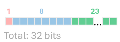
Floating point 32 (FP32)
Let me introduce how the Floating point number is organized in the example of FP32. It contains 32 bits, where 1 bit indicates the sign, 8 bits define the Exponent and 23 bits define the Fraction.
Every value V is defined by the formula:
For further reading, I refer you to the Wiki.
It’s important to note that FP32 can handle values up to \(10^{38}\) and precision up to ~\(7.2\) digits.
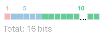
Floating point 16 (FP16)
The next format is FP16, which is half of FP32. It has 16 bits, where 1 bit indicates the sign, 5 bits define Exponent and 10 bits define Fraction.
Every value V is defined by the formula:
It’s important to note that FP16 can handle values up to \(10^{5}\) and precision up to ~\(3.3\) digits. Thus the precision is worse and the range is smaller than in FP32.
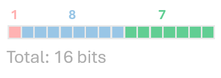
Brain floating point 16 (BF16)
BF16 is a special case of FP16, where the exponent is 8 bits and the fraction is 7 bits. This format can handle values up to \(10^{38}\) same as FP32 but precision only up to ~\(2\) digits.
Every value V is defined by the formula:
Floating point 8 (FP8)
The next format is FP8, which is half of FP16. It has 8 bits, and two versions: E5M2 and E4M3. The latter is subjectively more popular. E5M2 consists of 1 bit indicating the sign, 4 bits for Exponent, and 2 bits for Fraction. E4M3 consists of 1 bit indicating the sign, 3 bits for Exponent, and 3 bits for Fraction.E5M2 can handle values up to \(10^{5}\) and E4M3 - up to \(10^{3}\). For more information, you can find here.
Summary on formats
| Format | Bits | Sign | Exponent | Fraction | Max value | Precision |
|---|---|---|---|---|---|---|
| FP32 | 32 | 1 | 8 | 23 | \(10^{38}\) | ~7.2 |
| FP16 | 16 | 1 | 5 | 10 | \(10^{5}\) | ~3.3 |
| BF16 | 16 | 1 | 8 | 7 | \(10^{38}\) | ~2 |
| FP8 (E5M2) | 8 | 1 | 4 | 2 | \(10^{5}\) | ~2 |
| FP8 (E4M3) | 8 | 1 | 3 | 3 | \(10^{3}\) | ~2 |
Simple network and number recognition
Let’s create a simple network that recognizes numbers from 0 to 9. We will use the MNIST dataset. The network will consist of 2 convolutional layers and 2 fully connected layers. The network will be trained on the MNIST dataset and then we will quantize it to different formats.
import torch
from torchvision import datasets, transforms

class SimpleNN(torch.nn.Module):
    def __init__(self):
        super(SimpleNN, self).__init__()
        self.fc1 = torch.nn.Linear(784, 256)
        self.fc2 = torch.nn.Linear(256, 128)
        self.fc3 = torch.nn.Linear(128, 64)
        self.fc4 = torch.nn.Linear(64, 10)

    def forward(self, x):
        x = x.view(x.shape[0], -1)
        x = torch.nn.functional.relu(self.fc1(x))
        x = torch.nn.functional.relu(self.fc2(x))
        x = torch.nn.functional.relu(self.fc3(x))
        x = torch.nn.functional.log_softmax(self.fc4(x), dim=1)
        return x

transform = transforms.Compose(
    [transforms.ToTensor(), transforms.Normalize((0.1307,), (0.3081,))]
)

# Download and load the training data
trainset = datasets.MNIST("mnist_data", download=True,
train=True, transform=transform)
trainloader = torch.utils.data.DataLoader(trainset,
batch_size=64, shuffle=True)

# Download and load the test data
testset = datasets.MNIST("mnist_data", download=True,
train=False, transform=transform)
testloader = torch.utils.data.DataLoader(testset,
batch_size=64, shuffle=False)

model = SimpleNN()

byte_size = sum(p.element_size() * p.nelement() for p in model.parameters())
print(
    "Total size of the model: ",
    byte_size / 1_000_000,
    ' MB',
)
Total size of the model: 0.971048 MB
Let’s check the format:
for name, param in model.named_parameters():
    print(f"{name} is loaded in {param.dtype}")
fc1.weight is loaded in torch.float32
fc1.bias is loaded in torch.float32
fc2.weight is loaded in torch.float32
fc2.bias is loaded in torch.float32
fc3.weight is loaded in torch.float32
fc3.bias is loaded in torch.float32
fc4.weight is loaded in torch.float32
fc4.bias is loaded in torch.float32
In order to cast the model parameters to FP16, we can use the following code:
model_fp16 = model.half()
print(
    "Total size of the model: ",
    sum(p.element_size() * p.nelement()
    for p in model_fp16.parameters()) / 1_000_000,
    ' MB',
)
for name, param in model_fp16.named_parameters():
    print(f"{name} is loaded in {param.dtype}")
Total size of the model:  0.485524
fc1.weight is loaded in torch.float16
fc1.bias is loaded in torch.float16
...
Thus by using FP16, we reduced the size of the model by 50%. The same can be done with BF16 and FP8.
model_bf16 = model.to(torch.bfloat16)
print(
    "Total size of the model: ",
    sum(p.element_size() * p.nelement()
    for p in model_bf16.parameters()) / 1_000_000,
    ' MB',
)
for name, param in model_bf16.named_parameters():
    print(f"{name} is loaded in {param.dtype}")
Total size of the model:  0.485524 MB
fc1.weight is loaded in torch.bfloat16
fc1.bias is loaded in torch.bfloat16
...
For FP8 we have two options: E5M2 and E4M3.
model_fp8_e4m3fn = model.to(dtype=torch.float8_e4m3fn)
model_fp8_e5m2 = model.to(dtype=torch.float8_e5m2)
The size of the model is the same for both formats:
Total size of the model: 0.242762 MB
Thus by using FP8 we reduced the size of the model by 75%. But these are floating point formats.
Let’s test the difference in accuracies between the original model and the quantized models.
model = SimpleNN()
criterion = torch.nn.CrossEntropyLoss()
optimizer = torch.optim.Adam(model.parameters(), lr=0.01)

def train(model, trainloader, valloader, criterion, optimizer, epochs=5):
    train_losses = []
    val_losses = []
    for e in range(epochs):
        # Training step
        model.train()
        running_loss = 0
        progress_bar = tqdm(trainloader, desc=f"Epoch {e+1}/{epochs}")
        for images, labels in progress_bar:
            optimizer.zero_grad()
            output = model(images)
            loss = criterion(output, labels)
            loss.backward()
            optimizer.step()
            running_loss += loss.item()
            progress_bar.set_postfix(loss=running_loss / len(trainloader))
        train_loss = running_loss / len(trainloader)
        train_losses.append(train_loss)
        print(f"Training loss: {train_loss}")

        # Validation step
        model.eval()
        val_running_loss = 0
        with torch.no_grad():
            for val_images, val_labels in valloader:
                val_output = model(val_images)
                val_loss = criterion(val_output, val_labels)
                val_running_loss += val_loss.item()

        val_loss = val_running_loss / len(valloader)
        val_losses.append(val_loss)
        print(f"Validation loss: {val_loss}")

    return train_losses, val_losses

train_losses, val_losses = train(model,
trainloader, testloader, criterion, optimizer)
plt.plot(train_losses, label="Training loss")
plt.plot(val_losses, label="Validation loss")
plt.legend()
plt.show()
This code trains the model on the MNIST dataset. Now let’s test the accuracy of the model on the test dataset.
def test(model, testloader):
    correct = 0
    total = 0
    with torch.no_grad():
        for images, labels in testloader:
            outputs = model(images)
            _, predicted = torch.max(outputs.data, 1)
            total += labels.size(0)
            correct += (predicted == labels).sum().item()
    print(f"Accuracy of the model" \
        f"on the 10000 test images: {100 * correct / total}%")

test_model(model, testloader)
Accuracy of the model on the 10000 test images: 94.71%
To test the model casted to FP16 we also have to cast the test images to FP16.
testloader_fp16 = [(images.half(), labels) for images, labels in testloader]
model_fp16 = copy.deepcopy(model).half()
test_model(model_fp16, testloader_fp16)
Accuracy of the model on the 10000 test images: 94.72%
Unfortunately, I don’t have access to H100 or hardware that support FP8 to measure accuracy with FP8, but I hope the idea is clear. However, I’d like to show also inference on the test image.
def test_inference(data_loader, dict_models, ind):
    dataiter = iter(data_loader)
    images, labels = next(dataiter)

    img = images[ind]
    img = img / 2 + 0.5  # unnormalize
    npimg = img.numpy()
    plt.imshow(np.transpose(npimg, (1, 2, 0)))
    plt.show()
    for tag, model in dict_models.items():
        model.eval()

        # Move the model to the appropriate device
        model = model.to(device)

        # Move the image to the correct device and precision based on the model
        img_input = images[ind].unsqueeze(0).to(device)  # Add batch dimension

        # Handle different precisions
        if tag == 'BF16':
            img_input = img_input.to(dtype=torch.bfloat16)
        elif tag == 'FP16':
            img_input = img_input.to(dtype=torch.float16)
        else:  # FP32, default
            img_input = img_input.to(dtype=torch.float32)

        # Model inference
        with torch.no_grad():
            output = model(img_input)

        # Get the predicted class
        predicted_class = torch.argmax(output, dim=1).item()
        ground_truth = labels[ind].item()
        print(f"Prediction of {tag} model is " \
            f"{predicted_class}, ground truth is {ground_truth}")

test_inference(testloader,
{'FP32':model, 'BF16':model_bf16, 'FP16':model_fp16},
1)
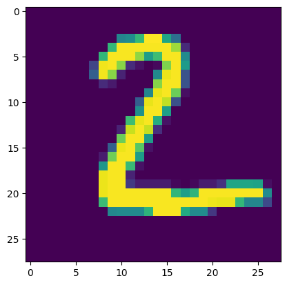
Prediction of FP32 model is 2, ground truth is 2
Prediction of BF16 model is 2, ground truth is 2
Prediction of FP16 model is 2, ground truth is 2
Real-world example
The example above is small and simple, ideal for grasping a concept. In daily life, we are dealing with much larger models. Let’s consider a BLIP model Salesforce/blip2-opt-2.7b from Hugging Face, link.
Let’s get our hands dirty and test it to FP16.
model = Blip2ForConditionalGeneration.from_pretrained("Salesforce/blip2-opt-2.7b",
    torch_dtype=torch.float16, device_map="auto")
url = "http://images.cocodataset.org/val2017/000000039769.jpg" # was 9
raw_image = Image.open(requests.get(url, stream=True).raw).convert('RGB')

# show image
plt.imshow(raw_image)
plt.show()

processor = Blip2Processor.from_pretrained("Salesforce/blip2-opt-2.7b")

question = "Describe what is in the picture?"
inputs = processor(images=raw_image,
return_tensors="pt").to("cuda", torch.float16)
with torch.no_grad():
    with torch.autocast(device_type="cuda", dtype=torch.float16):
        out = model.generate(**inputs)
print(processor.decode(out[0], skip_special_tokens=True).strip())
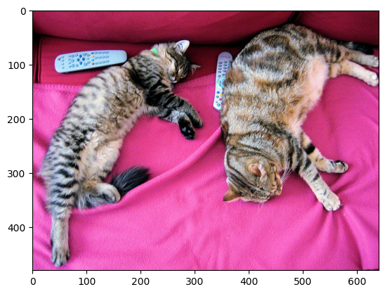
two cats laying on a couch
If we run !nvidia-smi, we can see that the model is running on the GPU and the memory usage:
+---------------------------------------------------------------------------------------+
| NVIDIA-SMI 535.104.05             Driver Version: 535.104.05   CUDA Version: 12.2     |
|-----------------------------------------+----------------------+----------------------+
| GPU  Name                 Persistence-M | Bus-Id        Disp.A | Volatile Uncorr. ECC |
| Fan  Temp   Perf          Pwr:Usage/Cap |         Memory-Usage | GPU-Util  Compute M. |
|                                         |                      |               MIG M. |
|=========================================+======================+======================|
|   0  Tesla T4                       Off | 00000000:00:04.0 Off |                    0 |
| N/A   64C    P0              47W /  70W |   7837MiB / 15360MiB |     66%      Default |
|                                         |                      |                  N/A |
+-----------------------------------------+----------------------+----------------------+

+---------------------------------------------------------------------------------------+
| Processes:                                                                            |
|  GPU   GI   CI        PID   Type   Process name                            GPU Memory |
|        ID   ID                                                             Usage      |
|=======================================================================================|
+---------------------------------------------------------------------------------------+
We see it takes 7.8 GB of memory. Let’s check what would be the output and the usage if we use the FP32 version.
model32 = Blip2ForConditionalGeneration.from_pretrained(
    "Salesforce/blip2-opt-2.7b",
    torch_dtype=torch.float32, device_map="auto"
    )
url = "http://images.cocodataset.org/val2017/000000039769.jpg"

raw_image = Image.open(requests.get(url, stream=True).raw).convert('RGB')
processor = Blip2Processor.from_pretrained("Salesforce/blip2-opt-2.7b")

question = "Describe what is in the picture?"
inputs = processor(images=raw_image,
return_tensors="pt").to("cuda", torch.float32)
with torch.no_grad():
    with torch.autocast(device_type="cuda", dtype=torch.float32):
        out = model32.generate(**inputs)
print(processor.decode(out[0], skip_special_tokens=True).strip())
two cats laying on a couch
Same as before. Let’s check the memory usage.
+---------------------------------------------------------------------------------------+
| NVIDIA-SMI 535.104.05             Driver Version: 535.104.05   CUDA Version: 12.2     |
|-----------------------------------------+----------------------+----------------------+
| GPU  Name                 Persistence-M | Bus-Id        Disp.A | Volatile Uncorr. ECC |
| Fan  Temp   Perf          Pwr:Usage/Cap |         Memory-Usage | GPU-Util  Compute M. |
|                                         |                      |               MIG M. |
|=========================================+======================+======================|
|   0  Tesla T4                       Off | 00000000:00:04.0 Off |                    0 |
| N/A   74C    P0              44W /  70W |  13451MiB / 15360MiB |     38%      Default |
|                                         |                      |                  N/A |
+-----------------------------------------+----------------------+----------------------+

+---------------------------------------------------------------------------------------+
| Processes:                                                                            |
|  GPU   GI   CI        PID   Type   Process name                            GPU Memory |
|        ID   ID                                                             Usage      |
|=======================================================================================|
+---------------------------------------------------------------------------------------+
The memory usage is 13.5 GB, which is almost twice as much as the FP16 version. This is a significant difference. You can imagine that in some cases you can’t even load the FP32 version of the model on the GPU. Moreover, for training, it needs more memory, for instance, this model in the FP16 version would need 28.9 GB.
Conclusion
In this post, we discussed different floating point formats and how to cast a model into a different format. We also showed how to train a simple network on the MNIST dataset and how to quantize it into different formats. Additionally, we demonstrated how to test the accuracy of the model on the test dataset and how to make inferences on a single image. Then we also showed how to load a real-world model in FP16 and FP32 and how to test the accuracy and memory usage of the model.
For the convenience of the reader, the full code can be found in the Google colab notebook here.
I hope you enjoyed this post and learned something new. If you have any questions or suggestions, please feel free to reach out to me on LinkedIn. Thank you for reading!